Friction Loss Along Pipe
- Pages: 11
- Word count: 2715
- Category: College Example Mechanical Engineering
A limited time offer! Get a custom sample essay written according to your requirements urgent 3h delivery guaranteed
Order NowAbstract
This experiment of the friction loss along a smooth pipe shows that there are existence of laminar and transitional flows as stated in Graph 2.0 and Graph 2.1. It is proven that the higher velocity along the smooth bore pipe, the higher is the head loss of water. As shown in Table 3.0, when the Reynolds’ number increases, the value of pipe coefficient friction, f decreases along the decreasing stead laminar line. On top of that, there are energy loss from the water to the surface of the pipe and therefore, the temperature increases when velocity, flow rate and head loss increases respectively. The percentage difference of obtained head loss and calculated head loss are 2.5%, 19.0%, 32.0%, 27.0% and 30.0% whereby the differences are not major and in the acceptable range. There are few factors in affecting the head loss which are flow rate, inner diameter of the pipe, roughness of the pipe wall, corrosion and scale deposits, viscosity of the liquid, fittings and also straightness of the pipe. There are existence of both human errors, parallax errors and environmental effect but there are always error counters to be taken place to increase the accuracy of the results.
Introduction
Basically, friction loss refers to the loss of energy which occurs in the pipe flow due to viscous effects generated by the surface of the 3mm ID pipe. It is understandable that friction loss is a major loss rather than minor loss including energy lost due to obstructions. Loss of head occurred by the mixing of fluid which occurs at fittings such as bends or valves, and also frictional resistance at the pipe wall. Besides, the major part of the head loss will be due to the local mixing near the fittings.
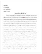
Figure 1.0 Illustration of Fully Developed Flow along a Pipe
Based on the figure above shows how the flow goes along the length of 0.52m with 3mm ID pipe which can be found in our experiment. Those fittings such as valves or bends are sufficiently remote to reduce any disturbance from them to ensure the distribution of velocity across the pipe does not vary with the length of the pipe. This flow is known as a “fully developed”. The head loss depends on the wall shear stress, τ in between the fluid and pipe surface. On top of that, the shear stress of a flow is also dependent on
whether the flow is turbulent or laminar.
Nevertheless, the Reynolds number is provided by
Re = =
whereby Q shows volumetric flow rate and the shows the molecular viscosity. This quantity varies with temperature whereby the higher the head loss of water and mercury, the higher the change in temperature. The Reynolds number determines whether the flow is laminar or turbulent. For a smooth pipe, the Re < 2100 shows laminar flow properties while Re > 4000 signifies turbulent flow properties. On the other hand, transitional flows refer to range 2100 < Re < 4000.
Figure 1.1 Laminar and Turbulent Flows Along a Pipe
Illustrations above shows the flows of laminar and turbulent properties along a smooth pipe whereby velocity increases from zero (minimal) at the wall to a maximum value U at the centre of the pipe. Therefore, the mean velocity, V is of course less than U in both flows. In laminar flow, the velocity profile is parabolic and the ratio U/V of the centre line velocity to mean velocity is = 2
Meanwhile, the velocity distribution is much flatter over most of the pipe cross section for the turbulent flow. The flatness of the profile is proportional to the Reynolds’ number whereby the ratio of maximum to mean velocity reduces slightly.
Graph 1.0 Graphs of h against u and log h against log u
The graphs shown above relates on how velocity, v along the pipe affects the head loss, h of both water and mercury. It increases steadily shows the existence of laminar flow then follow by random curves which represents transitional flow for both graphs. Besides, for graph of h against u has a curvy increase after the transition flow shows the existence of turbulent flow while a steady increase for graph of log h against log u.
Objectives
To determine the relationship between head loss due to fluid fraction and
velocity for flow of water through smooth bore pipe. To confirm the head loss predicted by pipe friction equation associated with flow of water through a smooth bore pipe. Apparatus
1. Holding Tank
2. Water Manometer
3. Mercury Manometer
4. Control Valve
5. Baseboard
6. Inlet Valve
7. Thermometer
Experimental Procedures
A. General Start Up
1. The water is filled into the sump tank of the Hydraulic Bench until approximately 90% full. 2. The water supply is connected from the Hydraulic Bench to Fluid Friction Measurement Apparatus using flexible hose. 3. A flexible hose is connected to the outlet and made sure that it is directed into the volumetric tank. 4. The outlet flow control valve is fully opened at the apparatus and the water flow is directed through the test section by switching the valves. 5. The bench flow control valve, V1 is fully closed then the pump is switched on. 6. V1 is opened gradually and the piping is allowed to fill with water until all air has been expelled from the system.
B. Experiment 1: Fluid Friction in Smooth Bore Pipes
1. The appropriate valves are opened and closed to obtain flow of water through the required test pipe. 2. The flow rates are measured using the volumetric cylinder in conjunction with flow control. 3. The head loss is measured between the tapping using the mercury monometer or pressurized water manometer as appropriate. 4. The readings are obtained on test section.
Results
A. Raw Results
Volume, V
(m3)
Time, T
(sec)
Head Loss, H
(mmHg)
Head Loss, h
(mH2O)
Temperature, T
(oC)
0.0002
167
21
0.04
31.0
0.0002
52
26
0.09
48.0
0.0002
40
30
0.14
52.0
0.0002
34
35
0.19
60.0
0.0002
29
38
0.25
61.0
Table 1.0 Raw Results Obtained
Diameter of the Pipe: 3 mm ID Smooth Bore Pipe
Initial Temperature: 27.0 oC
B. Calculated Results Based From Raw Results
Flow Rate, Q
(m3/s) x10-6
Velocity,
u
(m/s)
Log u
Log h
Temperature Difference, ∆T
(oC)
1.20
0.17
0.77
1.40
4.0
3.85
0.54
0.27
1.05
21.0
5.00
0.71
0.15
0.85
25.0
5.88
0.83
0.08
0.71
33.0
6.90
0.98
0.01
0.60
34.0
Table 2.0 Calculated Results
C. Calculated Results By Using Formulae And Moody Chart
Reynolds No., Re
λ
Calculated Head Loss, h
(mH2O)
Percentage Difference, %
443
0.360
0.09
2.5
1407
0.184
0.47
19.0
1850
0.176
0.78
32.0
2163
0.120
0.73
27.0
2554
0.100
0.85
30.0
Table 3.0 Formulae and Moody Chart Based Results
D. Graph of Head Loss against Velocity
Graph 2.0 Graph of head loss against velocity
E. Graph of log h against log u
Graph 2.1 Graph of log h against log u
F. Calculations
A sample calculation will be performed in this section; therefore, the first set of raw results will be taken into this section with a volume of 0.2-L. 1. To determine flow rate, Q.
Time, T = 167 sec
Volume, V = 0.2-L x
= 0.0002 m3
Flow rate, Q =
=
= 1.20 x 10⁻⁶ m3/sec
2. To determine velocity, u.
Flow rate, Q = 1.20 x 10⁻⁶ m3/sec
Diameter of the pipe = 3-mm x
= 0.003-m
Velocity =
=
= 0.17 m/s
3. To determine log u and log h.
Velocity, u = 0.17-m/s
Head loss for water, h= 0.04 mH2O
Log u = Log 0.17
= |-0.77|
= 0.77
Log h = Log 0.04
= |-1.40|
= 1.40
4. To determine the change in temperature, ∆T.
Initial temperature = 27oC
Obtained Temperature = 31oC
Change in temperature, ∆T = Obtained temperature – Initial Temperature
= (31 – 27) oC
= 4 oC
5. To determine the Reynolds’ number, Re .
Density, = 999 kg/m3
Velocity, u = 0.17 m/s
Molecular viscosity, = 1.15 x 10⁻³ Ns/m2
Diameter, d = 0.003-m
Reynolds’ number, Re =
=
= 443
6. To determine calculated head loss of water, h.
From the moody diagram,
Pipe coefficient friction, f = 0.09 (refer to the Moody Chart attached) Length, L = 0.52-m
Gravity, g = 9.81-m/s2
Diameter, d = 0.003-m
Velocity, u = 0.17-m/s
Head loss of water, h =
=
= 0.09 mH2O
7. To determine the percentage difference of obtained and calculated values of head loss of water. Obtained head loss of water, h = 0.04-m
Calculated head loss of water, h = 0.09-m
Percentage Difference, PD = x 100%
= x 100%
= 2.5% Discussion
The experiment is about the friction loss along a pipe and also to determine whether it is a laminar, transitional or turbulent flow by determining the Reynolds’ number as shown in the results part. Besides, it is also to determine the head loss in terms of height of mercury, mmHg and height of water, mH2O so does the temperature change and other respective observations which are necessary for this experiment.
Based on the results obtained from the results section, the volume is remained constant at 0.0002-m3 with five readings as stated in Table 1.0. Besides, we can notice that when the head loss of water increased from 0.04-mH2O to 0.25-mH2O requires lesser time from 167 seconds to 29 seconds respectively. This shows that when the head loss of water increases, the time requires collecting 0.0002-m3 reduces. In this experiment, the head loss water is the variable constant whereby flow rate of water is the responding variable. On top of that, it is sure that when the height of water increases will affect the height of the mercury as well but based on results obtained, the height of water is higher than the height of mercury.
The diameter of the smooth pipe is constant throughout the experiment which is 3-mm (0.003-m) and the experiment was started with an initial temperature of 27oC. As noticed, the flow rate of the water increases with respect to the height of water from 1.20 x 10⁻⁶ m3/s to 6.90 x 10⁻⁶ m3/s and this also affect the velocity of water along the smooth pipe increases initially from 0.17-m/s to 0.98-m/s. By referring to the formula P = hg whereby the density, and gravity, g remained constant due to same liquid which is water was used. Therefore, the pressure, p is proportional to height, h. A greater height leads to higher pressure and water flows from low to high pressure will increase the flow rate of the water. In this experiment, we controlled the height of water and determine the flow rate of water along the pipe whereby a more precise and contented results obtained.
The initial temperature water from the tank is 27oC, and when the obtained flow rate is 1.20 x 10⁻⁶ m3/s then the temperature is 31 oC with an increment of 4 oC. The final flow rate is 6.90 x 10⁻⁶ m3/s with the temperature of 61 oC, an increment of 34 oC. There is an increase in temperature because of the energy loss whereby the change in velocity will cause the change in energy transfer rate. Basically, the energy lost by the liquid is converted to heat energy by friction because the amount of liquid enters and exits must have the same amount and therefore, the velocity along the pipe must be equal. If the velocity is constant then the velocity energy (head) must be equal/constant as well. Therefore, the pressure energy is the only energy left besides velocity energy. The measured pressure entering the pipe will be higher than the measured pressure exiting the pipe. On top of that, value of Log u and Log h are determined whereby the values increased from -0.77 to -0.01 and -1.40 to -0.60 respectively.
Then, moving on to the calculated Reynolds’ number and calculated head loss by using formulas. Based on Tables 2.0 and 3.0 under result section showed that when the velocity increases, the Reynolds’ number increases as well whereby the flow rate of water plays an important role as well. At velocity of 0.17-m/s has Reynolds’ number of 443 and at velocity of 0.98-m/s has Reynolds’ number of 2554. In Table 3.0, there are existences of two flows which are laminar and transitional flows. The velocities of 0.17-m/s, 0.54-m/s and 0.71-m/s have Reynolds’ number of 443, 1407 and 1850 respectively which fall into laminar flow (Re < 2100). On the other hand, the velocities of 0.83-m/s and 0.98-m/s have Reynolds’ number of 2163 and 2554 respectively which shows that they inhibit transitional flow (2100 < Re < 4000) properties. Besides, the value of lambda, λ is plotted and obtained through Moody’s chart and being inserted at the back part of the report. The value of lambda decreases with respect to Reynolds, number increases because they are in laminar and transitional flow.
The calculated head losses of water are 0.09-mH2O, 0.47-mH2O, 0.78-mH2O, 0.73-mH2O, and 0.85-mH2O respectively and comparisons are made with the obtained head loss of water whereby percentage differences do exist which is 2.5%, 19%, 32%, 27%, and 30% respectively. The sample calculations are inserted in Part F under result section to ease readers out in terms of calculations and understanding. Based on the percentage difference obtained, the differences are not huge enough and still in the acceptable range. The calculated head loss would be an ideal one because assumptions were made instead of obtained head loss values which have affecting factors.
There are few factors which affect the head loss which are flow rate, inner diameter of the pipe, roughness of the pipe wall, corrosion and scale deposits, viscosity of the liquid, fittings and also straightness of the pipe. Based on graph 2.0 shows the a steady increase for the laminar flow from velocity of 0.17-m/s to 0.71-m/s then there is a slightly curvy line created which signifies the existence of transitional flow with velocity from 0.83-m/s to 0.98-m/s. In this graph, turbulent flow is cannot be shown because the highest Reynolds’ number in this experiment is 2554 which lies in transitional flow region. Therefore, the graph has laminar and transitional flows only. On top of that, referring to Graph 2.1 which is graph of Log h against Log u whereby the laminar flow has a straight and elevated line then follow by a curvy look line of graph which shows transitional flow. Therefore, this graph inhibits the same properties as Graph 2.0 whereby only existences of laminar and transitional flow.
There are existences of errors in every experiment and therefore errors were arisen in this experiment as well. That is why; the obtained results and calculated results have percentage difference. Firstly, parallel errors arise when the eye of the observer is not parallel to the designated readings and slightly elevated from the designated point, therefore, deviations happen. Secondly, the height of the water, mH2O is not precise and the values obtained are slightly more or less and bring to the nearest value. That is why, percentage errors arise. Thirdly, the thermometer is not allowed to dip into the water for some time instead removed in a count of five. Last but not least, the Pipe-Friction Apparatus is not equipped with analog gauges or manometers instead of manual manometers.
Every error has its own solution to improve the results obtained from the experiment. Firstly, in order to prevent parallax error, the eyes of the observer must be parallel to the designated readings on the manometer to achieve 100% accurate readings. Secondly, we must jot down the actual value on the manometer instead of bringing to the nearest value. This would increase the accuracy and decrease the discrepancy of results. Thirdly, the thermometer must dip into the water for some time to achieve stable state of heat transfer and therefore, a more favorable temperature could be obtained. Last but not least, by setting up analog manometers or gauges onto the Pipe-Friction Apparatus would ease the observers and also able to determine the values with higher precision and prevent errors.
Conclusions
The objectives have been fulfilled and proven on the experiment shown above. There are existence of laminar flow and transitional flow in this experiment whereby Re < 2100 and 2100 < Re < 4000 respectively. The percentage difference for all the readings are minor which are 2.5%, 19%, 32%, 27%, and 30% respectively. Therefore, there is an existence of friction along the smooth pipe.
References
1. n.a. (February 9, 2013). STA-RITE, Pentair Water. In Head Loss in Piping Systems. From http://www.sta-rite.com/ResidentialPage_techinfopage_headloss.aspx. 2. n.a. (August 4, 2013). Pipe friction loss. Retrieved February 8, 2013, from http://www.jfccivilengineer.com/pipe_friction_loss.htm. 3. Wikipedia. (January 23, 2013). Friction loss. In Wikipedia, The Free Encyclopedia. Retrieved February 7, 2013, from http://en.wikipedia.org/wiki/Friction_loss. 4. n.a.. (February 6, 2013). Laboratory #8 – Head Losses in Pipe Flow. In CE 319F. From http://www.ce.utexas.edu/prof/kinnas/319LAB/Lab/Lab%208-Head%20Losses%20in%20


