Economics of the environment
- Pages: 34
- Word count: 8335
- Category: Economics Environment Supply and Demand
A limited time offer! Get a custom sample essay written according to your requirements urgent 3h delivery guaranteed
Order Now1.Research on the admission fees to national parks has found that the price elasticity of demand for annual visits to Glacier National Park is 0.2. The National Park Service is now considering a 10-percent increase in the admission fee. a)What will happen to the number of annual visits to Glacier National Park? Solve for a numerical answer. Ep = % Δ Q/ % Δ P
0.2 = % Δ Q / 10%
% Δ Q = 2%
b)Will the revenues that the park collects increase or decrease? Briefly explain. The total revenues at the park would increase after an increase in price if the demand was inelastic or decrease after an increase in price if the demand was elastic. As the demand can be considered inelastic (given that Ep <1), I would expect the park revenues to increase. 2.Which has a greater elasticity: a supply curve that goes through the origin with a slope of 1 or a supply curve that goes through the origin with a slope of 4? Please graph and explain.
A supply curve that goes through the origin with a slope of 1 has unitary elasticity – meaning a percentage change in price will lead to a similar percentage change in the quantity supplied. Eg. [(15-10)/(15+10)] / [(15-10)/(15+10)] = 1
For the supply curve with a slope of 4, the same is true if the curve goes through the origin. Eg. [(2-1)/(2+1)] / [(8-4)/(8+4)] = [1/3] / [1/3] = 1
Or [(5-3)/(5+3)] / [(20-12)/(20+12)] = [1/4] / [1/4] = 1
Any linear supply curve that passes through the origin will have unitary elasticity (Es = 1), where a percentage change in the price will lead to an equivalent percentage change in the quantity. 3.When the price of tents rises by 15 percent, the demand for backpacks falls by 1 percent. a)Calculate the cross price elasticity of demand.
Exp = [(Q2a – Q1a)/ (Q2a + Q1a)] / [(P2b – P1b)/ (P2b + P1b)] = -1%/15%
= – 0.07
b)Are the goods complements or substitutes?
As Exp <0, these goods are complements.
c)By how much would demand for backpacks have to rise for the goods to switch from complements to substitutes, or vice versa? If the percentage change in the quantity demanded was a positive instead of a negative (ie. a rise in demand instead of a fall), the goods could be considered substitutes. I’m not sure if you’re asking for the percentage change from the new state (ie. after a fall of 1%) or not. For the new state, you’d need an increase of over 101.01%. 4.A political leader comes to you and wonders whom she will get the most complaints if she institutes a price ceiling when demand is inelastic and supply is elastic. a)How do you respond?
Assuming the price ceiling was set at below the equilibrium price, a new equilibrium would occur where the amount of goods supplied would be less than the amount of goods originally demanded. Producers or suppliers in this case would complain the most since the price ceiling would result in a decrease in overall producer surplus. In addition, there might also be complaints from consumers if they are not able to access the good. I’m assuming here that an inelastic demand curve indicates the good may be a necessity with limited substitutes. In some cases (depending on the good), a black market could arise, where those with money or connections are able to purchase the good at a higher price. In this case, the suppliers might take in more money and poorer people would be hurt the most (with subsequent complaints). b)Demonstrate why your answer is correct.
At the price ceiling imposed, sellers will only be willing to produce a certain quantity (Qc), which is much less than the quantity demanded (Qd) at that price. This is a shortage (Qd – Qc) that will cause complaints by both the buyers and sellers. If we consider the original producer surplus (triangle P*CE), we see that it will decrease after the ceiling is imposed to triangle FDE. If we consider the original consumer surplus (ACP*), it is ambiguous whether the new consumer surplus will be higher or lower (ABDF). The producers would be unhappy with this change due to the decrease and a subset of the buyers would likely be unhappy as well (depending on how the good is distributed).
5.Consider the market for hiking boots. This market can be represented by the following supply and demand equations: Q = 800 – 400P (demand) and Q = – 50 + 100P (supply)
a)Graph the supply and demand curves, labeling the axes clearly. Calculate the equilibrium price and quantity in this market (Q represents a pair of boots), and label these points on the graph.
Equilibrium price is $1.70 and equilibrium quantity is 120 pairs of boots. b)Calculate consumer surplus, producer surplus, and social welfare in the market for hiking shoes.
CS = 1/2*(120*(2-1.7)) = 18
PS = 1/2*(120*(1.7-0.5)) = 72
TS = social welfare = CS + PS = 90
c)Now suppose that a tax of 50 cents is imposed on each pair of boots. With the tax of 50 cents, find the price that consumers pay, the price that firms receive, and the quantity exchanged.
After the tax of 50 cents, consumers will pay a new price of $1.80 for a pair of boots, sellers will receive a price of $1.30, and the quantity exchanged will lower from 120 pairs of boots to 80 pairs of boots. d)Calculate the total tax revenues. How much of the tax incidence falls on consumers? And how much of the tax incidence falls on producers? Total tax revenues
= Q * tax rate
= 80 * 0.5
= $40
To calculate the tax incidence, find the difference between the old equilibrium price and the after tax price. In this case, the consumers pay $0.10 (or 20% of the tax – $8 total) and the producers pay $0.40 (or 80% of the tax- $32 total). e)Calculate consumer surplus, producer surplus, and the level of social welfare associated with the tax.
CS = 1/2*((80)*(2-1.8)) = $8
PS = 1/2*((80)*(1.3-0.5)) = $32
TS = social welfare = CS + PS + tax revenues
= $40 + $40
= $80
f)Calculate the deadweight loss associated with the tax.
DWL = TS (pre tax) – TS (post tax)
= $10
Consider the market for hiking boots. This market can be represented by the following supply and demand equations: Q = 800 – 400P (demand) and Q = – 50 + 100P (supply)
a)Graph the supply and demand curves, labeling the axes clearly. Calculate the equilibrium price and quantity in this market (Q represents a pair of boots), and label these points on the graph.
Equilibrium price is $1.70 and equilibrium quantity is 120 pairs of boots. b)Calculate consumer surplus, producer surplus, and social welfare in the market for hiking shoes. CS = 1/2*(120*(2-1.7))
= 18
PS = 1/2*(120*(1.7-0.5))
= 72
TS = social welfare = CS + PS
= 90
c)Now suppose that a tax of 50 cents is imposed on each pair of boots. With the tax of 50 cents, find the price that consumers pay, the price that firms receive, and the quantity exchanged.
After the tax of 50 cents, consumers will pay a new price of $1.80 for a pair of boots, sellers will receive a price of $1.30, and the quantity exchanged will lower from 120 pairs of boots to 80 pairs of boots. d)Calculate the total tax revenues. How much of the tax incidence falls on consumers? And how much of the tax incidence falls on producers? Total tax revenues = Q * tax rate
= 80 * 0.5
= $40
To calculate the tax incidence, find the difference between the old equilibrium price and the after tax price. In this case, the consumers pay $0.10 (or 20% of the tax – $8 total) and the producers pay $0.40 (or 80% of the tax- $32 total). e)Calculate consumer surplus, producer surplus, and the level of social welfare associated with the tax. CS = 1/2*((80)*(2-1.8))
= $8
PS = 1/2*((80)*(1.3-0.5))
= $32
TS = social welfare = CS + PS + tax revenues
= $40 + $40
= $80
f)Calculate the deadweight loss associated with the tax.
DWL = TS (pre tax) – TS (post tax)
= $10
2)Indicate whether each of the following activities is associated with a positive externality, a negative externality, or neither. Briefly explain your answers. a)Someone at your table is chewing with his or her mouth open. It will depend, but I’ll say this may constitute a negative externality. If the people around are caused some type of harm/annoyance by the person’s behaviour, it would be considered a negative externality. b)Going to graduate school in environmental management.Neither – there’s the potential for positive externalities to come out of the education if you work on public issues after you graduate, but there isn’t anything inherent in the pursual of the degree that would make it either a positive or negative externality. c) Someone comes unprepared to a study group.
Negative externality as the individual is imposing a cost, either in time or stress/annoyance on the others without doing anything themselves. They would end up benefitting from the activity without paying the cost. d)Someone is scalping tickets to the US Open at a ridiculously high price. Neither. This could indicate a shortage of tickets, but if people are willing to pay the price, it’s up to them. e) Someone asks a really good question in class.
Positive. Everyone benefits from the question and answer, including the person that asked the question. f)The European Union signing the Kyoto Protocol.Possibly positive, if it influences other bodies to sign on and the EU actually follows through on whatever their commitments are. g)Driving your car.Negative due to the emissions associated with driving a car (assuming they aren’t paid for in some way). 3)In class, we showed that for goods associated with a negative production externality, the efficient quantity of exchange is lower than that which is determined by the market. Demonstrate graphically that the opposite holds with a positive externality. In other words, show graphically that for goods associated with a positive externality (assume a production externality), the efficient quantity of exchange is higher than that which is determined by the market. Carefully label your graph with all parts necessary to make your case.
In the case of a positive production externality, the marginal social cost of the production is not taken into account to compensate producers. In this case, the original supply curve (MC) and demand curve (MWTP) meet at equilibrium point A (given a price of P* and quantity demanded of Q*). When the marginal social cost is taken into account (curve MSC), it can be seen that the new equilibrium would be reached at point B (at a price P’ and a quantity Q’). This would allow a net increase in welfare (equivalent to DWL in the graph) and the quantity demanded would be higher than the original market (ie. Q’ > Q*).4)The daily market for gasoline is characterized by the demand curve Q = 10 – P and the perfectly elastic supply curve P = 2, where Q = millions of gallons per day and P = price/gallon. The burning of gasoline generates pollution and creates an externality. Economists estimate the externality to be $2 per gallon. a.Construct a graph that includes the demand curve, the supply curve, and the social marginal cost (SMC) curve. b.Assuming no government policies, solve for the equilibrium quantity and the efficient quantity. Label them both on your graph. Equilibrium quantity is where S meets D, at quantity 8.
Efficient quantity is where SMC meets D, at quantity 6.
c.On your graph indicate the deadweight loss (DWL) that will arise without
government intervention. DWL occurs when social cost is not taken into account and is indicated by the coloured triangle below. (DWL = ½ (2*2) = 2) d.Suppose a Pigouvian tax is proposed to correct the market failure. How much should the tax be per gallon? The tax should be set at $2 per gallon (equivalent to the social costs of the externality). e.Calculate the tax revenue that the Pigouvian tax would generate. Label it on the graph. The revenue generated would equal the tax multiplied by the quantity consumed per day. It would equal 6,000,000 x 2 = $12,000,000/day.
f.With the tax in place, calculate total surplus (TS). Label it on the graph. Total surplus = Consumer surplus + producer surplus + tax generated – pollution cost Consumer surplus = area below the demand curve at the given price Producer surplus = 0 (receiving the same amount as marginal cost) tax generated = tax rate * quantity (=12)
pollution cost = pollution cost * quantity (=12)
So, TS = CS
1/2 (6*6) = 18
g.What, if any, are the remaining pollution costs to society? The costs associated with the pollution (per unit pollution cost of $2 multiplied by the quantity) were offset by the tax instituted. Total pollution costs were $12,000,000, which were offset by an equivalent tax of $12,000,000. 1.The daily market for dry-erase markers on campus is characterized by the following inverse demand and supply curves Inverse demand: P = 5 – Q
Inverse supply: P = 3
a.Sketch the graph of the demand and supply curves.
b.Solve for the equilibrium price and quantity, label it on the graph. P = 5 – Q
P = 3
3 = 5 – Q
Q = 2, P = $3 (Assume dollars)
c.Solve for consumer surplus, producer surplus, and total surplus, labeling
all on the graph as appropriate. CS = ½ (2*2) = 2
PS = 0 (receiving same price as marginal cost)
TS = CS + PS = 2
d.Now assume that the “off-gassing” of each marker creates a negative health externality. But it is not known how to value the marginal external cost per marker. What is the minimum external cost per marker that would imply zero markers is the efficient quantity? If we’re assuming zero markers are the efficient quantity, then the minimum external cost required would be the difference between the original cost at quantity 0 and the cost along the demand curve for that quantity. ie.
Min external cost = P(5) – P* = 5- 3 =$2 per marker (assumed dollars)
e.Assuming your answer to part d is correct, solve for the deadweight loss of not regulating the market for dry-erase markers on campus, and label it on the graph. DWL = ½ (2*2) = 2
f.Is your answer to part e also equal to the total costs of pollution in the unregulated market? Briefly explain. If we’re assuming, as above, that the cost of health pollution is equal to $2, then the answer to part E does not equal the total costs associated with pollution in an unregulated market. Those costs would equal the pollution cost multiplied by the equilibrium quantity (ie. 2*$2 = $4). g.Would your answer to part e change if the marginal external costs were even greater? Briefly explain. Yes, if the marginal external costs were greater than the total area for the DWL would also increase, as per the diagram below.
2.TRUE / FALSE / UNCERTAIN
For these questions, you must argue your case (roughly 3 to 5 sentences) and make any assumptions necessary to compose your answer, including graphs if helpful. Points depend entirely on the quality of your explanation.a.When listening to a good song on the radio, there is no opportunity cost because it is free. False – The opportunity cost will be the value of the next best alternative to whatever you’ve chosen. In this case, the cost might be not listening to another good song on the radio. It doesn’t matter whether listening to the radio is free, as the cost might be in the form of something else – such as time in this case (ie. you can’t listen to both songs at the same time and may only have limited amount of time to listen to one song). b.Taxes always reduce economic efficiency.
False – taxes do not always reduce economic efficiency. Taxes can be used to shift towards greater efficiency when they target negative externalities (eg.a tax on carbon), especially when they’re used to offset other types of taxes (such as income taxes). c.Microeconomic theory implies that both population growth and rising per capita income in China will result in greater demand for automobiles in China. Probably true – If we assume that cars are a normal good, then microeconomic theory would indicate that rising income levels would increase the demand in China. It’s uncertain how the demand would change given the population growth occurring at the same time, and the greater pollutants associated with the greater demand for cars. It’s possible, though unlikely, that over time, other transportation options would be developed that would balance the need to travel greater distances with lower pollution profiles and higher densities (eg. high speed electric trains). So while it’s likely that the demand for cars would be greater, the effects of population and pollution might overtake the effects of rising income which could result in competing alternative technologies (hence the answer of probably true).
d.With a Pigouvian tax, tax revenue always equal the costs of pollution at the efficient condition. False – tax revenue is a function of the tax rate and the number of units produced. If the marginal cost of pollution increases at a greater rate than the marginal cost of production, the tax revenues generated will not necessarily account for the total costs of all pollution. In this case, tax revenues at the efficient condition would equal the area of ABCD, while pollution costs would be the area CDE (ie. the difference between the social marginal cost and the marginal cost for the efficient quantity). It’s not clear whether these two areas are equal. e.Whenever there is a consumption externality, equilibrium consumption will be inefficiently high. False – it depends on whether the externality is positive or negative. A negative externality will tend to overproduce (ie. equilibrium consumption will be inefficiently high) while a positive externality will tend to under-produce, with equilibrium consumption being inefficiently low. 3.Briefly describe the free rider problem in your own words using an example of a public good.
The free rider problem arises when someone is able to receive the benefits of a good without actually paying for them. If we take the case of a public good, such as national defense, we see it is both non-excludable (ie. a country will not exclude me from being defended in some way when I live there) and is also non-rival in consumption (ie. if I am defended, it’s also very likely that the people around me will be as well). However, I do not have to actually contribute to national defense in order to reap the benefits. As such, I could be considered a free-rider. 4.A neighborhood that consists of 100 individuals is trying to construct a communal flag pole, which will be a public good. They are trying to decide how high of a pole to construct. The price per foot of the pole is P = $10, and each individual has his/her own demand curve Q = 10 – P, which is the same for all individuals, and Q is the height measured in feet. What is the efficient height of the flag pole? Would you expect the individuals to voluntarily provide a flag pole at the efficient height? Briefly explain why or why not. For public goods, we can determine the efficient quantity by vertically summing all the individual demand curves. Assume P = 10 – Q for each person
For 100 people, SMB = 100(10-Q) = 1000 – 100Q
at P = 10,
100Q = 1000 – 10
Q = 9.9 ftI wouldn’t expect the individuals to voluntarily provide a flag pole at the efficient height. As this is the case of a public good, each individual has little incentive to provide for the flag pole as they can enjoy the benefits when other people pay (ie. there’s a positive externality enjoyed by all). In fact, we can see from the original individual demand equation (Q = 10 – P), that at a price point P = $10, the equilibrium quantity for each individual is actually 0. It is only when aggregate demand/benefits are taken into account do we see the efficient pole height. Suppose you are given the following supply curve: Q = 2 + 2P. What is the
price elasticity of supply for a price change from P = 4 to P = 5 (Use the midpoint formula)? Is supply elastic, inelastic, or unit elastic over this range? At P = 4, Q = 10. At P = 5, Q = 12
Elasticity = [(q2-q1)/(q2+q1)] / [(p2-p1)/(p2+p1)] = (2/22)/(1/9) = +0.81
Price elasticity of supply is inelastic (Es <1)
2. Explain why the equilibrium provision of a good that is both non-rival and non-excludible is suscep-tible to the free rider problem. Explain why this is a problem. If a good is non-excludable, it means a person cannot be stopped from benefitting from that good. If a good is non-rival, it means that a person’s use of that good does not diminish the use of that good for other people. If a good is both non-excludable and non-rival, it can be susceptible to the free rider problem, where people are able to obtain benefits from a good without feeling the need to pay for them (as they can’t be excluded from using it). This becomes a problem because it then becomes difficult to maintain the upkeep of these types of goods as the total level of voluntary provision for the goods will be inefficiently low. If we consider public goods to be the outcome of a positive externality (where social marginal benefit is greater than individual marginal benefit), people will be able to receive more benefits than they are actually willing to pay for, which would mean the good would be under-supplied.
As the good is also non-excludable, people would take advantage and be ‘free riders’ of the good. 3. Describe a good that is both rival and non-excludable, and explain whether (and why) you believe it is susceptible to the “Tragedy of the Commons.” Fisheries are an example of a good that could be considered rival and non-excludable. It would be difficult to effectively monitor and enforce certain fishing standards across the world (ie. the global fishing stock is non-excludable) but when certain fish (eg. blue-fin tuna) are fished by one person, other people are not able to obtain the same benefit due to stock depletion (ie. it is a rival good). This type of good would be susceptible to the “Tragedy of the Commons”, as people would believe they should catch the fish before someone else does. This would result in the fish being depleted at a higher rate than they can re-produce, resulting in an exploitation of the resource.
4. British Petroleum (BP) and Exxon-Mobile (EM) are both considering whether to increase their spend-ing on advertising to improve their “green” image. They each know their payoffs depend on what the other does. Payoffs are given in the matrix below. a. Identify the Nash equilibrium, clearly stating the equilibrium strategy of both BP and EM. BP
Raise SpendingStay the same
Raise spending
BP: $2 million
EM: $3 million
BP: $3 million
EM: $4 million
Stay the same
BP: $3 million
EM: $2 million
BP: $4 million
EM: $3 million
Exxon Mobil
From the perspective of BP:
-If Exxon raises spending, BP will stay the same
-If Exxon stays the same, BP will stay the same
From the perspective of Exxon:
-If BP raises spending, Exxon will raise spending
-If BP stays the same, Exxon will raise spending
Nash Equilibrium where BP will stay the same, and Exxon will raise spending. b. Carefully and briefly explain why the outcome in which both “Raise spending” is not a Nash equilibrium. The outcome where both BP and Exxon ‘raise spending’ is not an equilibrium is not a Nash equilibrium as BP has a better strategy at that point given Exxon’s action. If Exxon raised spending, BP would actually gain more benefit ($3mill as opposed to $2mill) by keeping their advertising budget the same. As the definition of a Nash equilibrium is when all actors choose their strategy given the strategy chosen by all other actors, and there is no incentive to change their behaviour, this would not be considered a Nash Equilibrium. 5. Construct a graph to characterize the market for paper. Assume there is a negative production externality that comes from the manufacturing of paper. On your graph be sure to label the following: a) all curves and axes, b) the efficient quantity, c) the equilibrium quantity, d) the marginal external cost, e) the total pollution costs at the equilibrium quantity, and f) the deadweight loss. PMSC
S = MC
P*
D=MWTP
Q’Q*Q
Efficient quantity at Q’
Equilibrium quantity at Q*
Marginal external cost at MSC curve
Total pollution costs = triangle ACD
Deadweight loss = triangle BCD
6. Construct a graphical argument that shows why domestic consumers are likely to be in favor of free trade in goods for which their country is at a comparative disadvantage. Using the same graph(s), indicate why domestic firms that manufacture the good are likely to hold the opposite position. P
S = MC(country)
P*
P’S = MC(world)
D=MWTP(country)
Q*Q’Q
In this case, the marginal cost to produce goods in a certain country is shown by the S=MC(country) curve. The marginal cost for the production of these goods in other parts of the world is less and shown in the curve S=MC(world). Consumers would want to be paying the lower world price (P’ as opposed to P*). The total consumer surplus in this case would increase from domestic production (CS = ABG) to the much larger ACF. Domestic
manufacturing firms would lose out on total surplus in this case, going from PS=GBE to PS=FDE .7. Consider a perfectly competitive market for laptop computers. It can be represented by the following equations for supply and demand: Q = 4P – 4000 (supply) Q = 6000 – P (demand) a.Graph the supply and demand curves, labeling the axes and the x- and y- intercepts. b.Calculate the equilibrium price and quantity, and label them clearly on your graph. Supply
Q = 4P – 4000
P = 1/4Q + 1000
Demand
Q = 6000 – P
P = -Q + 6000
At equilibrium:
1/4Q + 1000 = -Q+6000
5/4Q = 5000
Q = 4000, P = 2000
c.Calculate the levels of consumer surplus, producer surplus, and social welfare in this market. CS = (1/2)(4000)(4000) = 8,000,000
PS = (1/2)(4000)(1000) =2,000,000
TS = CS + PS = 10,000,000
d.Assume the government is contemplating two possible price ceilings on computers: one at $2500 and one at $1500. Which one is binding? A binding price ceiling could be placed at $1500. This is lower than the market equilibrium price. If the ceiling was put at $2500, there would be no effect on the market (either quantity demanded or sold). e.Assume the government implements the binding price ceiling in part (d). On a new graph, illus-trate the equilibrium price and quantity that will arise in the market with the price ceiling in place. f.Solve mathematically for the initial shortage that will result with the price ceiling. Initial shortage would be the difference between the quantity demanded and the quantity supplied at the price ceiling price. At a price of $1500, quantity supplied would be 2000. While the quantity demanded would be 4500. The shortage would be 2500 units. g.On your graph, label consumer surplus, producer surplus, and total surplus with the price ceiling. (3 points) see graph
h. Calculate the deadweight loss associated with the price ceiling. DWL = (1/2)(2000)(2000-1500) + (1/2)(2000)(4000-2000) = 500,000 + 2,000,000 = $2,500,000
8. Suppose that tulip bulbs (flowers for planting) are produced and sold in a competitive market. Sup-pose further that people buy tulip bulbs to plant in front of their houses. The market demand curve for tulip bulbs is Q = 24 – P.
Suppose further that, completely unknown to those who plant tulip bulbs, people who pass their houses enjoy looking at the flowers. Specifically, the plants of tulips can be thought of a generating a positive consumption externality valued at $3 per planted tulip bulb. Finally, assume that the market supply curve for tulip bulbs is Q = 2P.
a. What is the equilibrium quantity of tulip bulbs bought and sold in the market? DemandSupply
Q = 24-PQ = 2P
P = 24 – QP = ½ Q
Eq 24-Q = 1/2Q
3/2 Q = 24
Q = 16, P = 8
j. Sketch a graph that shows total surplus at the market equilibrium? (Be sure to label all curves and intercepts) k. What would be the efficient number of tulip bulbs to be bought and sold in the market? Ef Q = 27-P, Q = 2P
27-Q = 1/2Q
3/2Q = 27
Q = 18, P = 9
l. What is the deadweight loss that society suffers from being at the
equilibrium quantity rather the efficient quantity? DWL = (1/2)(2)(1) + (1/2)(2)(2)
= $3
m. What Pigovian tax or subsidy could be employed to eliminate the deadweight loss? (You should specify whether it should be a tax or a subsidy, and you should specify the amount of the tax or subsidy.) A subsidy of $3 could be employed to eliminate the DWL. This subsidy would incentivize more tulips to be purchased and planted to eliminate the deadweight loss (by taking into account the social benefits gained by planting the tulips). . Consider the market for paper. The process of producing paper creates pollution. Assume the marginal damage function of pollution is given by MDF = 2E,
where damages are measured in dollars and E is the level of emissions. Assume further that the marginal abatement cost curve (expressed in terms of emissions) is MAC = 90 – E,
where costs are measured in dollars and E is the level of emissions. a)Graph the marginal damage function and the marginal abatement cost function. P* = 60, E* = 30
b)What is the unregulated level of emissions Eu?
Eu = 90 – where the MAC curve intercepts the x-axis
c)Assume an existing emission standard limits emissions to E = 50. Show on the graph why this policy is inefficient.
An emissions limit of 50 is greater than the efficient limit of E=30. At a limit of E=50, the marginal damages outweigh the costs of abatement, so the damage should be abated until it went to the efficient quantity of 30. d)Solve for the efficient emission standard. Assuming perfect compliance with this standard, what are the total costs of pollution? And what are the total costs of abatement? The efficient emission standard is at E = 30, where the MDF and MAC intersect. At this point, the total costs of pollution are:
= (0.5)(30)(60)
=$900
At this point, the total costs of abatement are:
= (0.5)(60)(60)
=$1800
e)If compliance with the standard becomes a problem, and you are able to set a fine for noncompliance, what would be the optimal fine per unit of emissions? The optimal fine would be the price at the optimal level of emissions, or P = 60. This assumes you’re actually able to fully enforce the fine at that level. If not, you need to determine some sort of probability the fine will actually be paid and increase the actual fine level to that point (although I don’t think you’re actually asking for that here). f)Now, rather than a standard, you are able to set a tax on emissions. At what level would you set the tax? How much revenue would the tax generate? Indicate the tax revenue on your graph. Set the tax at P = 60 (similar to the fine).
Tax revenue = (60)(30) = $1800
Tax revenue noted by shaded area above.
g)Now, rather than a standard or a tax, you are able to pay a subsidy for abatement. How much would you subsidize each unit of abatement? With this policy, what is the total subsidy payment? Indicate the subsidy payment on your graph. Subsidy would be set at P = 60.
Total subsidy payment = (60)(60) =$3600
2. Bill owns a coal fired power plant. There is currently a pollution tax of $4 per ton of SO2 emissions. Bill faces a marginal abatement cost function: MAC = 10 – (½)E, where E is his annual level of emissions. a. Calculate Bill’s (i) optimal level of annual emissions, (i) total abatement costs, and (iii) total tax payment to the government. Optimal emissions will be at intersection of tax curve and MAC 10-0.5E = 4
0.5E = 6
E = 12
Total abatement costs = (distance from unregulated emissions to regulated) x (costs) = (0.5)(20-12)(4) =$16
Total tax payment to government = tax x emissions at efficient quantity = (12)(4) =$48
b. Suddenly a new scrubbing technology becomes available and reduces the marginal cost of abatement. The scrubber only lasts one year. If Bill adopts the technology, he faces a new marginal abatement cost function: MAC’ = 8 – (½)E. What is the most Bill would be willing to pay to adopt the technology? With the new scrubber, the efficient level of emissions is” 8-0.5E=4
0.5E = 8
E = 4
His total costs would equal tax costs + abatement costs = (0.5)(16-8)(4) + (8)(4) =$48
Difference is:
48+16-48 =$16
Bill would be willing to pay up to $16 for the new system.
3. Consider a single firm that manufactures chemicals and generates pollution through its emissions E. Researchers have estimated the MDF and MAC curves for the emissions to be the following: D = 2E (MDF) and C = 90 – E (MAC), where D is damages and C is costs. Policymakers have decided to implement an emissions tax to control pollution. They are aware that a per unit tax of $60 is an efficient policy. Yet they are also aware that this policy is not politically feasible because of the large tax burden it places on the firm. As a result, policymakers propose a two-part tax: a per unit tax of $30 for the first 20 units of emissions,
then an increase in the per unit tax to $60 for all further units of emissions. a.Would the two-part tax be efficient? (Explain using a graph) Yes, it is efficient because companies would prefer to abate until the efficient emissions (E* = 30) as the abatement costs until that point are less than the costs of either levels of the tax. b.How much would the two-part tax save the firm compared to the constant $60 tax? Savings would be on the first 20 units of emissions.
Instead of a system with a tax of $60 per unit, where total = = (60)(3) =$1800
Total would be =
=(30)(20) + (10)(60)
=$1200
Savings would be $600
c. How would your answers to part (a) and (b) change if the jump from $30 to $60 occurred after the first 60 units of emissions rather than the first 20? If the change happened at E= 60, then the firm would likely emit to the point of E = 60 since it would be cheaper to pay the tax than the abatement costs. For part a) the firm wouldn’t reach the efficient emissions level of E = 30 (ie. they would emit more) for part b) the tax payment would be
= (60)(30)
= $1800
while a $60 tax would be
= (60)(60)
= $3600
so savings would be $1800
4. Consider the problem of choosing to implement an emission standard or an emission tax in a particular industry. Assume very good information is available about the marginal abatement costs. But there is much uncertainty about the marginal damages of emissions. In this situation, and from an economics perspective, which of the two policy instruments (standard or tax) would you chose to implement and why. In this case, where the MAC is known well, but there is uncertainty about the MDF curves, I don’t think it matters whether you use a tax or a standard. If you assume a certain MDF, and set either a tax or a standard, if the MDF is lower or higher, the total social loss will be the same for either the tax or the standard. This is because if the MAC is known, if either a tax or quantity of emissions is set, we’ll know where the corresponding point on the MAC is. See the following chart, where either a tax or standard is set at P1 (or E1) on MDF1. If the MDF is actually MDF2, the DWL will be the same whether you have set a tax or emissions standard.
1.If you were head of the Environmental Protection Agency, would you be more interested in your economic advisors’ positive views or their normative views? Briefly explain why. I would be more interested in their positive views, however I’d also be interested in the normative views of my economic advisors. Understanding their positive views would allow me to have a better understanding of the facts about the given policy under consideration, which could then be tested or modified in some way. Understanding their normative views would also be beneficial, as they would help reveal any biases the advisors might have (which would help in assessing their interpretation of the data being presented) as well as giving me a better understanding of the possible choices that could be made subjectively given the set of information being analyzed. 2.An environmental organization is trying to decide on the best way to spend the remainder of its annual budget. There are three possible choices: (a) use the money for more fundraising, (b) increase lobbying expenditures, and (c) support more grassroots organizing.
For accounting purposes, the organization must spend all of its remaining budget on only one of the three possible choices. Assume the organization has chosen to go with more fundraising. What is the “opportunity cost” of this decision? Briefly explain. If the organization has chosen to spend the remainder of their budget on fundraising, the opportunity cost can be considered the potential net benefit they would not realize of one of the remaining two options. It’s hard to say which of the two remaining options would be more beneficial to the organization since there’s no information given as to the possible outcomes of each activity, but as an example, if increased lobbying efforts would provide more benefits than grassroots organizing, then the opportunity cost would be the net benefit of the lobbying activities.
A similar comparison could be made if grassroots organizing was determined to provide more marginal benefits than increased lobbying efforts. 3.For each of the following markets, indicate whether the stated change causes a shift in the supply curve (a change in supply), a shift in the demand curve (a change in demand), a movement along the supply curve (a change in quantity supplied) or a movement along the demand curve (a change in quantity demanded). Clearly state any assumptions you make in drawing your conclusions. a)The housing market: consumers’ incomes increase.
Assuming that real estate in the housing market can be considered a normal good, an increase in consumers’ incomes would also see an increase in demand (i.e. a shift of the demand curve to the right). b)The camera market: the price of film goes up.
Assuming that we’re talking about film cameras, and that film and cameras can be considered complementary products, the increase in the price of film would cause a decrease in demand of cameras (i.e. they are related products). c)The sugar market: there is a drought in the sugar cane fields in Florida. The drought would cause a decrease in the supply of sugar (i.e. a shift in the supply curve to the left). d)The milk market: the price of milk increases, and the amount of milk people are willing to buy declines. Assuming a market in equilibrium, a decrease in the amount of milk people are willing to buy (i.e. a shift in the quantity demanded) would cause a decrease in the amount of milk being supplied to the market, which would also (eventually) lower the price of milk. e)The video rental market: the number of consumers in the area decreases. Assuming there’s a relationship between the number of consumers in a given area and the number of videos that are rented, if the number of consumers in the area decreases, then the demand for video rentals would also decrease (i.e. a shift in the demand curve to the left). f)The ice cream market: the price of frozen yogurt falls.
Assume that frozen yogurt is a substitute for ice cream. When the price of frozen yogurt falls, the demand for frozen yogurt will increase, and the demand for ice cream will decrease (i.e. a shift of the ice cream demand curve to the left). This also assumes both are normal goods. 4.Suppose you are given the following information about the market for bottles of water: Q = 120-10P (market demand) and Q = 50P (market supply), where P = price per bottle, and Q = quantity of bottles.
a)Graph the demand and supply curves for bottles of water. Clearly label both axes, as well as the y-intercepts for each curve.
b)Solve algebraically for the equilibrium price and quantity in the market for bottles of water. Eq1 : Q1 = 120-10P1
Eq2 : Q2 = 50P2
At equilibrium, Eq1 = Eq2,
120-10P = 50P
60P = 120
P = 2
Substitute into Eq2, Q = 100
Equilibrium price (P*) is $2 and equilibrium quantity is 100. c)What will happen to the equilibrium price and quantity in this market for each of the following changes? Sketch a graph comparing the old and new equilibria, and clearly state any assumptions you make in drawing your conclusions i)The price of soda increases.
Assume normal goods and that soda is a substitute for bottled water. An increase in the price of soda would lead to an increase in the demand for bottled water. If the supply of bottled water stays the same, the price of water, as well as the quantity demanded will increase.
ii) Income increases.
Assuming bottled water is a normal good, an increase in income would correspond with an increase in the demand for bottled water (i.e. a shift of the demand curve to the right) – similar to the example above. The quantity demanded and the price would increase.
iii) The price of the plastic used in producing water bottles increases. Assuming a normal good. Higher priced plastic would increase the marginal cost of production of bottled water, meaning the supply curve would shift to the left. The quantity demanded would decrease and the prices for bottled water would increase.
5.The basis of microeconomic theory is the notion of thinking at the margin (not marginal thinking!). Accordingly, it is helpful to interpret a demand curve as a marginal benefit curve, and to interpret a supply curve as a marginal cost curve. Using these interpretations, briefly explain why the intersection of a demand curve and a supply curve gives rise to an equilibrium price and quantity. A demand curve can be considered a marginal benefit curve – indicating a person’s willingness to pay for a certain quantity of a good. For each increase in price, the marginal benefit derived decreases. Similarly, a supply curve can be considered a marginal cost curve that shows the costs associated with producing a good. In terms of equilibrium, if the quantity demanded was higher than the natural equilibrium quantity (given a certain price), a supplier would not be willing to produce that much supply, since it would require a marginal cost greater than the price they were receiving (i.e. they would be losing money). Consumers, on the other hand, wouldn’t be willing to pay an increased price as they wouldn’t be receiving enough marginal benefit from doing so. In this way, both the quantity demanded and quantity supplied would move towards the equilibrium point, where the marginal costs borne by producers and marginal benefits received by consumers would be equal.
6.Recent research indicates an alarming increase in drug use among young people. In the ensuing debate, various reasons for the increase have been given. Two of these are (i) fewer police officers patrolling the streets have resulted in increased availability of drugs, and (ii) drug use is once again considered cool among a new generation of teenagers. a)Use supply and demand diagrams to show how each of the explanations above could lead to an increase in the quantity of drugs consumed. Case 1 – fewer police officers patrolling the streets would lead to a change in the supply of drugs as the marginal cost of drugdealing would decrease, assuming things like the cost of lookouts and people going to jail are incorporated into the total costs. This means that for the same price, more drugs could be sold, and eventually a new equilibrium would be reached where a higher quantity of drugs were sold at a lower price than the initial state (assuming constant demand curve).
Case 2 – if drugs were cool again (oh – the horror!), the perceived marginal benefit would increase, which would lead to a change in the demand for drugs (i.e. a shift in the demand curve to the right). This means that for the same price, a higher quantity of drugs would be demanded, leading to more drugs being sold at a higher price than the initial state (assuming constant supply).
b)How could information about what has happened to the price of drugs help to distinguish between these explanations? If we assume either a constant demand in case 1 or a constant supply in case 2, we can determine which explanation is most likely depending on the price of drugs. In both cases, there is an increase in the quantity of drugs being sold, however a decrease in price would result from a change in the supply, while an increase in price would indicate a change in the demand. 7.Please visit the Environmental Performance Index webpage put together at Yale. Url: http://epi.yale.edu/. Searching around the website you will find the “Data Explorer” and also access to raw data files to use if you like. Looking at the relationship between different indices (e.g., overall performance, or different sub-measures as discussed in class) and GDP/capita, do you find evidence in support of the notion that environmental quality is a normal good?
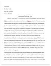
Does the pattern hold across all measures of environmental performance? Please explain and also include at least one graph using EPI data in your answer, and limit your written to response to one page of text. Some answers will be selected for very brief presentation in class. If environmental quality is a normal good, then citizens in countries with higher GDP per capita would presumably demand a ‘higher quality’ environment, which could be indicated by higher performance scores on an environmental index (amongst other things). Looking at the overall performance scores from the 2014 edition of Yale’s Environmental Performance Index, we can see this seems to hold true to an extent – those countries with higher GDP per capita appear to also have higher performance scores on the index.
Source: Environmental Performance Index 2014, Yale University When considering different aspects of environmental performance, this seems to hold true for certain factors. The EPI chart below shows household air quality per country against GDP per capita. Similar to the overall EPI performance score, it seems that countries with higher GDP also have higher household air quality scores.
Source: Environmental Performance Index 2014, Yale University However, this isn’t the case for all criteria that the EPI tracks. Below is a chart showing critical habitat protection versus GDP, and as can be seen, there are quite a few countries with higher GDP (inc. Canada, the US and Japan) that have lower scores than those that might be anticipated for countries that might be concerned with the environment.
To be honest, it’s very difficult to draw any sort of conclusion from the EPI charts, probably because they are static in time. While environmental quality may be considered a normal good, and while it may follow a so-called Environmental Kuznets Curve (where degradation increases up to a certain point while income increases until environmental protection kicks in), the data provided can’t really be used to make a conclusion because we’re comparing one country to another, when in fact, environmental management decisions are most likely to be made within countries (or regions). As such, it would be much more beneficial to look at historic environmental data of a certain country over a specific time period to understand the effect of an increase in GDP and its relationship on environmental quality. Fortunately, some studies have already been completed in this area. Below is a link to three graphs, each showing sulphur emissions per capita from Canada, Botswana and Brunei from the years 1850-2000. As can be seen by the Canada graph, there does appear to be an increase in environmental quality over time as GDP per capita increases (or at least a decrease in sulphur emissions which relate to things like acid rain, smog, etc.).
However, the same cannot be said for Botswana. Of course, this could be due a lower limit required for GDP prior to any change in environmental quality. When looking at Brunei, we can see a similar relationship as observed in Canada over the same time period (to a certain extent). This is not to say that the Kuznets curve isn’t valid – it’s more likely the theory holds for certain countries, but under specific conditions and for certain environmental criteria. In the case of sulphur, it’s likely that an easy technological solution (eg. scrubbers) or specific policy could be used to manage a pollutant which had visible local or regional effects (eg. smog or acid rain). In the case of other environmental criteria, such as carbon dioxide, forest cover, etc., there may be other factors that need to be considered in addition to GDP. Some of these factors may include good governance structures, strong civil societies, higher rates of education, etc. Although it is likely that these factors also occur in countries with higher GDP levels, it would be difficult to make any real conclusions without further study.


